What Role Does an Acoustic Model Play in Speech Recognition?

All resources

Rev › Blog › Resources › Other Resources › A.I. & Speech Recognition › What Role Does an Acoustic Model Play in Speech Recognition?

Automatic speech recognition systems are complex pieces of technical machinery that take audio clips of human speech and translate them into written text. This is usually for purposes such as closed captioning a video or transcribing an audio recording of a meeting for later review. ASR systems are not monolithic objects, but rather are composed of two, distinct models: an acoustic model and a language model.

The acoustic model typically deals with the raw audio waveforms of human speech, predicting what phoneme each waveform corresponds to, typically at the character or subword level. The language model guides the acoustic model, discarding predictions which are improbable given the constraints of proper grammar and the topic of discussion. In this article, we’ll go in depth on how acoustic models are constructed and how they integrate into the larger ASR system as a whole.

Challenges in Acoustic Modeling

There are multiple challenges involved in authentically modeling acoustic signals such as the audio waveforms of speech. The first is that waveforms are extremely nuanced. Not only do they pick up the sounds of speech, but they pick up background noise from the environment and other acoustic irregularities as well.

Each environment has its own acoustics – the sound of people speaking in an echoey church will be much different than that of speaking in a soundproof podcasting studio. Thus acoustic modeling is as much a signal processing problem as it is a modeling one, where the raw speech signal needs to be filtered out from the combination waveform.

The waveform of a given word or phoneme is also not uniform across individuals. Each person has a unique way of speaking, a different pitch and timbre to their voice, a slightly different way of annunciating, their own peculiar accent, and variations in the way they speak, from the use of slang to creating elisions of words.

Even the waveforms produced by a single individual constantly vary based on their tone of voice (angry, sad, happy, excited), the volume at which they speak, and myriad other factors. Thus a good acoustic model needs to have enough sensitivity to detect utterances of different phonemes but also not so much sensitivity that it can’t generalize broader patterns of speech across individuals. This is a classic issue in machine learning – the model must not be trained to overfit to one particular voice or style of speech.

Try Rev Ai Speech Recognition Free for Your First 5 Hours

Data Features in Acoustic Modeling

When working with acoustic models, we need to somehow featurize the raw audio waveforms, i.e. transform them into vector-valued quantities that the model can deal with. The key to doing this is to use techniques from classical signal processing.

These techniques also allow us to effectively handle many of the challenges described in the previous section, such as removing ambient noise and inconsistencies in speech across different speakers. Typically, signal processing features are captured using 25ms sliding window frames which are spaced 10ms apart. This allows the featurization process to capture useful features of the audio while at the same time ensuring that such features do not become too fine-grained.

Mel-Frequency Cepstral Coefficients

One common featurization method for audio uses what are called mel-frequency cepstral coefficients (MFCC). There is a lot of pre-processing work that goes into creating MFCCs. For example, a pre-emphasis stage is used to boost the intensity of higher frequencies within the signal. Next, the sliding windows are created. These are often computed using window functions, sometimes called Hamming and Hanning Windows, which more gently taper the boundaries of each window’s signal, allowing for higher downstream processing quality.

After this, a Discrete Fourier Transform (DFT) is applied to transform the signal from the time domain to the frequency domain. Then the outputs of the DFT are squared, giving the power of speech at each frequency. Finally, filter banks are computed by applying triangular filters to these power frequencies using a Mel scale. The Mel scale basically maps the signal in a way that is more consistent with the way humans naturally perceive sound. Our ears are more sensitive to lower than to higher frequencies, so the Mel scale adjusts the signal accordingly. The outputs of this step are called filter banks, and they themselves are often used as features to acoustic models.

Assuming that the MFCC is the desired feature type, however, we need a few additional steps. The problem with using raw filter banks is that they can sometimes be correlated, so the further processing used to compute MFCCs can help to negate some of that. To remove some of the correlation, we take the log of the Mel filter bank outputs and then apply a Discrete Cosine Transform (DCT) to the result.

The DCT is an orthogonal transformation which means that, in mathematical terms, it produces decorrelated outputs. The outputs of this DCT are called the cepstral coefficients, and typically we discard all of them except for 12, coefficients numbers 2-13. The remaining coefficients represent subtle changes in the filter banks which are typically not discriminative for acoustic modeling. Thus, it is usually safe to discard them.

MFCCs vs. Filter Banks

While MFCCs were quite popular with classical model types such as Hidden Markov Models and Gaussian Mixture Models, recent advances with neural networks and deep learning have shown that it is often possible to train on the raw filter banks. This is because deep neural networks are a more expressive model type and are less susceptible to correlations in the inputs.

Perceptual Linear Prediction

A third featurization method is called Perceptual Linear Prediction (PLP). This method proceeds in the same way as MFCC up to the mel filterbank step. At this point, the raw filter bank coefficients are weighted using an equal loudness curve and then compressed by taking the cubic root of the weighted outputs. Then a linear regression is used to compute coefficients for this loudness spectrum, and finally an inverse DFT such as the DCT is used as before to compute the cepstral coefficients. The advantage of the PLP method over MFCC is that it is slightly more robust to noise and gives slightly better overall accuracy in many cases.

In previous years, the primary models used for acoustic modeling were Hidden Markov Models (HMMs) and Gaussian Mixture Models (GMMs). They operated on a statistical framework based around maximizing the probability of the optimal word sequence given an input of raw audio waveforms. These days, deep learning models such as Neural Networks and Restricted Boltzmann Machines are the core drivers in innovation surrounding acoustic modeling and look to continue to be for some time to come.

Try Rev Ai Speech Recognition Free for Your First 5 Hours

HMM-GMM Model

In classical acoustic modeling, we are given an input X, for example MFCC features derived from a raw audio waveform, and we want to predict $W^*$ , the probabilistically optimal sequence of words obtained by the model having seen X. We can model this as

$W^* = \argmax_W P(W | X)$

By applying Bayes’ Rule, this gives us

$W^* = \argmax_W P(W | X) = P(X | W) * P(W) / P(X) = argmax_W P(X | W) * P(W)$

In that last step, we are able to remove $P(X)$ from the denominator because this probability is independent of $W$ , the variable which we are maximizing with respect to.

Now, in this scenario, we typically model $P(X | W)$ using the acoustic model and $P(W)$ given the language model. This is because the probability of W is independent of the acoustic features $X$ and instead has to do with a word’s probability in the natural use of language independent of the audio being presented.

A hidden markov model is represented as a set of states, a corresponding transition matrix giving the probability of moving between any pair of states, a set of observations, and a set of emission probabilities of an observation being generated from a given state. In HMMs for speech recognition, the states are phonemes, i.e. units of sound used in the articulation of words, and the observations are the acoustic feature vectors given by MFCCs or similar.

HMM models for speech are generally left-to-right, i.e. they place strong priors on transition probabilities such that certain phonemes can only occur after others and that the HMM cannot backtrack to previous states. This type of constrained HMM is called a Bakis network and is constrained due to how rigorously constructed human speech is. Such a network also allows self loops, allowing a phoneme to repeat in case its utterance duration is greater than the 25ms window width.

The next step in constructing the HMM model requires us to estimate the observation probabilities $o_t$ of seeing one of the observed acoustic MFCC vectors. Since we don’t have access to these probabilities, we often make the assumption that they follow a multivariate Gaussian distribution

$\frac{1}{2\pi}^{D/2} |\Sigma |^{1/2} \exp \left( -\frac{1}{2} (o_t - \mu_j)^T \Sigma^{-1}_j (o_t - \mu_j) \right)$

where $o_t$ is the observation vector at time $t$ , $\mu_j$ is the mean vector of the observations and D is the dimensionality of the observations. $\Sigma$ is the diagonal covariance matrix with each entry along the diagonal corresponding to the covariance of a single observation vector dimension. Note how $\mu_j$ and $\Sigma$ are both readily computable from the observed data.

The GMM models the observation likelihoods as being drawn from a mixture of the above multivariate gaussian distributions. This mixture model and the HMM are trained jointly using a special case of the Expectation-Maximization (EM) algorithm called the Baum-Welch algorithm.

Substituting Neural Networks

The past ten years or so have seen a shift to replacing the GMM in the HMM-GMM acoustic model with various Deep Neural Network (DNN) models. Because DNNs are so good at discriminative learning, particularly when trained on sufficiently sized datasets, they have given much improved accuracy over GMM models for modeling the observation probabilities $o_t$ .

In the early 2010s, models such as Restricted Boltzmann Machines and Deep Belief Networks were popular choices for the DNN. These days, however, sequence based models such as LSTMs, Bidirectional-LSTMs, or GRUs are most frequently used. What’s more, these models are normally trained directly on the Mel filter bank features directly rather than the MFCCs, offering as advantages reduced preprocessing time and richer feature representations.

Using bidirectional layers gives close to the current state of the art. The bidirectionality is useful because it allows the model to consider both the left and right contexts of any given observation and improves overall modeling accuracy. A current state of the art configuration for the DNN model looks something like the below:

LSTM with 4-6 bidirectional layers with 1024 cells/layer (512 each direction)
256 unit linear bottleneck layer
32k context-dependent state outputs
Input features:
- 40-dimension linearly transformed MFCCs (plus ivector)
- 64-dimension log mel filter bank features (plus first and second derivatives)
- concatenation of MFCC and filter bank features
Training: 14 passes frame-level cross-entropy training, 1 pass sequence training (2 weeks on a K80 GPU)

LSTMs + feature fusion currently reach close to state-of-the-art.

Rev AI’s Acoustic Modeling

While a naively trained acoustic model might be able to detect well-enunciated words in a crystal clear audio track, it might very well fail in a more challenging environment. This is why it’s so important for the acoustic model to have access to a huge repository of (audio file, transcript) training pairs.

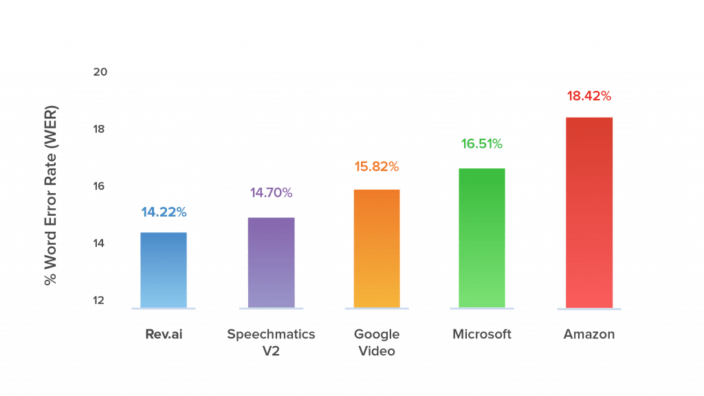
This is one reason why Rev’s automatic speech recognition excels. It has access to training data from 10+ years of work of 50,000 native English speaking transcriptionists and the corresponding audio files. This is something even the largest companies don’t have, and it allows Rev to beat Google, Microsoft, Amazon, and more tech giants in speech recognition accuracy.

Try Rev Ai Free for Your First 5 Hours

More Caption & Subtitle Articles

Closed Captioning	Add Captions in Premiere Pro
Add Closed Captions to Videos	Zoom Closed Captioning
Add Captions to YouTube Videos	Add Captions to TikTok Videos
Add Captions to Vimeo Videos	Add Subtitles to MP4 Videos
What is an SRT File?	Add Captions to iMovie